Basics Of Statistics & Why Should You Care About Median And Mode


This blog is the first of a series about statistical concepts that every Data Science/Machine Learning beginner should learn. In this part, we are going to discuss the very basic concepts of statistics, stuff that almost everyone has learned at some point during their school or college time. So treat this as a brief refresher, go through it quickly and see if you know everything, do pay attention to the Measures of Dispersions you might just learn something new and interesting.
Facts are stubborn things, but statistics are pliable ~ Mark Twain
Let's say we are working as data analysts at a fintech start-up and we've just been handed the credentials to their database. What do we do with it? Do we just start making a bunch of fancy reports about the data? No. First, we need to understand what the data can tell us about the business and see if this information can be leveraged to solve any existing problems.
Another thing we can do is draw insights from the data, but what are insights?
Insight is valuable knowledge obtained by analyzing data. This definition is rather vague and broad, and that is so for a reason. A lot of things can fall under the category of insights - what ad campaign will be more effective, what portions of a supply chain are slowing down the logistics network, what category of expenses is the most wasteful, what is the likelihood of a defective product in a particular manufacturing batch, etc.
Descriptive Statistics
But the problem is that it is not possible to understand something by simply glancing at the data in most cases. Even while working with a thousand data points it is not feasible to go through each of them individually and look for patterns. To make the process of drawing insights and making assumptions easier; the data needs to be summarized by a set of easily interpretable values or attributes.
That is where descriptive statistics come in, they are used to condense the information into a few easy to use data points. There are two sets of descriptive statistics -
- Measures of Central Tendency: They are used to summarize the most common or most "central" value of an attribute. For example, the average height or weight of a group of people.
- Measures of Dispersion: They describe the variations in an attribute. For example, the normal blood pressure or heartbeat range.
Before we get into the different measures let's quickly understand a very fundamental classification of data: Qualitative vs Quantitative
Qualitative & Quantitative Data
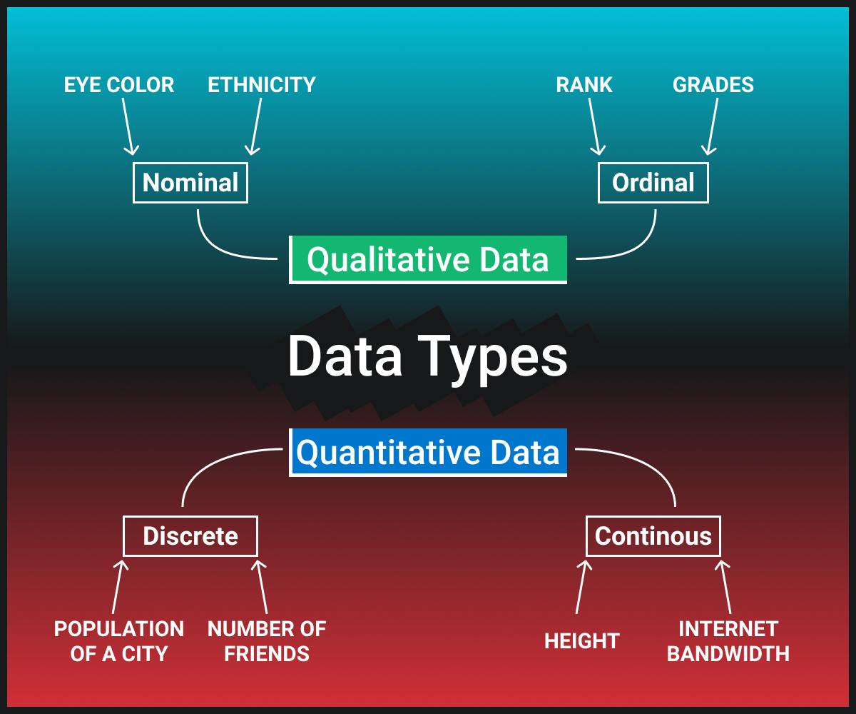
Quantitative Data
Quantitative Data, as the name suggests, consists of mathematical values that indicate a quantity, amount, or measurement of a property. When we deal with quantitative measures, the numbers mean themselves. That is, there is no additional information required: 4.2 is 4.2 and 100 is 100.
Discrete data scale is one that is quantitative but does not take up all the space. Let's take the number of siblings as an example — we may have 1 sibling, 3 siblings, 5 siblings, or even 10, but we cannot have .5 or 4.25.
Continuous scale on the other hand takes up all the space, it can be anything from -∞ to +∞, can be fractional. For example, we can measure time in days, hours, seconds, milliseconds and so on. The continuous scale is determined throughout all possible values.
Qualitative Data
Qualitative Data reflects the properties or qualities of objects. Numbers here don't mean themselves, but they signify some qualities or properties of objects. In other words, they serve as markers for some categories. For example, let's say we compare people living with different colors of eyes. We can encode people with blue eyes by 1, black eyes by 2, and so on. Here 1,213... don't mean anything except that they denote these categories.
Qualitative variables are divided into nominal and ordinal types. Let's take a closer look at what each of these types means, starting with nominal variables. The only information nominal variables contain is information about an object belonging to a certain category or group. It means that these variables can only be measured in terms of belonging to some significantly different classes, and you will not be able to determine the order of these classes.
For example, we earlier considered the example of people with different colors of eyes — blue eyes, green eyes, brown eyes. These categories will all be nominal variables — there is no order in these values.
Ordinal variables differ slightly from nominal variables by the fact that there is an order to the category, a preference. So, values not only divide objects into classes or groups but also order them. For example, we have grades at school — A, B, C, D, F. And in this case we can say for sure that the person who got an A is probably more prepared for the test than the person who received an F. In this case, we cannot say to what extent, but we can say for sure that A is better than D.
Measures of Central Tendency
To understand the various measures of central tendency let's create some data that we can use to illustrate the different measures.
data = [5, 6, 8, 9, 1, 2, 8, 4, 6, 2, 4, 8, 6, 1]
Mean
Mean, or more specifically the arithmetic mean is the first statistical measure we are taught in school. It is given by

def mean(x):
    return sum(x) / len(x)

mean(data)

4.23076923076
Median
The median for the data arranged in increasing order is defined as :
- If n is an odd number - The middle value
- If n is an even number - Mean of the two middle values
def median(data):
    n = len(data)
    sorted_data = sorted(data)
    midpoint = n // 2
    if n % 2 == 1:
        # if odd, return the middle value
        return sorted_data[midpoint]
    else:
        # if even, return the average of the middle values
        low = midpoint - 1
        high = midpoint
        return (sorted_data[low] + sorted_data[high]) / 2

median(data)

4
Mode
The mode is the most commonly occurring data value. May have more than one value.
def mode(x):
    counts = Counter(x)
    max_count = max(counts.values())
    return [x_i for x_i, count in counts.iteritems() if count == max_count]

mode(data)

6
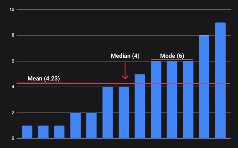
Why do we need all three?

Consider the distribution of household income in the U.S. Commonly, when we discuss income or want to compare the income of two places, we use the median income. This is the income level below which half of the households earn. This is indicated on the plot, as about $50,000 (in 2010). This is a useful measure of the general "location" of "central tendency" of the data. You can imagine if we wanted to discuss the general income of say New Jersey vs. Kansas, that the median is a useful statistic. The median is useful for skewed data, like this income data, or for data with outlying values.
The mode isn't indicated on the plot, but it is clearly the $15000 - $19999 category. This tells you something different about the data, basically that more than any other category, more households earn $15000 - $20000.
Finally, the mean is useful for symmetric data. In skewed data, it is influenced by outlying values. So, in the case of this income data, it would likely be considerably higher than the 50,000 median, because the few households with extremely high incomes pull up the average. This might misrepresent the general income level.
A general framework for deciding when to use what:
| Type of Variable | Optimal Measure of Central Tendency |
| Nominal | Mode |
| Ordinal | Median |
| Quantitative(not skewed) | Mean |
| Quantitative(skewed) | Median |
Measures of Dispersion
Range
The range is the difference between the smallest and the largest data points in the sample.
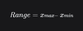
max(data) - min(data)
8
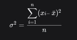
Variance
Variance measures how far data points are distributed from the mean of the sample. It is the average of the squared differences from the Mean.
import numpy as np
np.var(data)
7.0
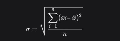
Standard Deviation
Standard deviation is the square root of the variance.
import numpy as np
np.std(data)
2.6457513110645907
What is the need for standard deviation?
A question now arises, if the standard deviation is just the square root of the variance why do we need to calculate it? After all, the variance does a decent enough job of describing the distribution of the data. Here's why:

The variance of a data set measures the mathematical dispersion of the data relative to the mean. However, though this value is theoretically correct, it is difficult to apply in a real-world sense because the values used to calculate it were squared. The standard deviation, as the square root of the variance, gives a value that is in the same units as the original values, which makes it much easier to work with and easier to interpret in conjunction with the concept of the normal curve.
Measure the dispersion of height (cm) in terms of area (cm^2), doesn't make sense now, does it? There are other reasons (and uses) for calculating the standard deviation, we'll talk about these later when discussing statistical tests and normal distributions.
What's the difference between variance and standard deviation?
Standard Deviation and Variance for Population and Sample data
Standard Deviation for Population
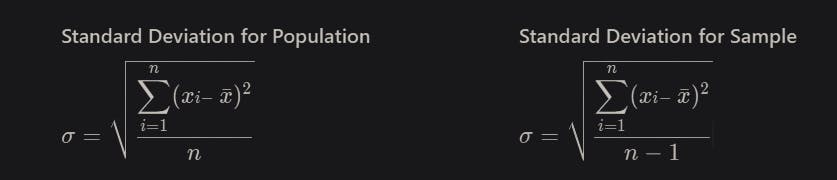
Similarly, we use "n-1" when calculating the variance using sample data
Why do we divide by n-1 instead of n?
Steps to calculate the standard deviation for a sample:
- Compute the square of the difference between each value and the sample mean.
- Add those values up.
- Divide the sum by n-1.
- Take the square root to obtain the Standard Deviation.
In step 1, we compute the difference between each value and the mean of those values. We don't know the true mean of the population; all we know is the mean of the sample. Except for the rare cases where the sample mean happens to equal the population mean, the data will be closer to the sample mean than it will be to the true population mean. So, the value you compute in step 2 will probably be a bit smaller (and can't be larger) than what it would be if we used the true population mean in step 1. To make up for this, we divide by n-1 rather than n.
This use of ‘n-1’ is called Bessel’s correction method.
Sample Standard Deviation vs. Population Standard Deviation
Inferential Statistics

Descriptive statistics provide us with information about the data sample we already have. For example, we could calculate the mean and standard deviation of SAT results for 50 students, and this could give us information about this group of 50 students. But very often we are not interested in a specific group of students, but in students in general - for example, all students in the US. Any sample of data that includes all the data we are interested in is called a population.
Very often it happens that we do not have access to the entire population in which we are interested, but only a small sample. For example, we may be interested in exam scores for all students in the US. It is not possible to collect the exam scores of all students, so instead, we will measure a smaller sample of students (e.g. 1000 students), which is used to display a larger population of all US students. But it is important that the data sample accurately reflects the overall population. The process of achieving this is called sampling(we will discuss sampling strategies in a later post).
Inferential statistics allow us to draw conclusions about the population from sample data that might not be immediately obvious. Inferential statistics emerges because sampling leads to a sampling error (what we accommodated for with Bessel’s correction), and therefore the sampling does not perfectly reflect the population. The methods of inferential statistics are:
- parameter estimation
- hypothesis-testing
We'll learn about these in later posts. That's it for now! 👋