In the first two parts of this series, we covered the fundamental concepts of statistics namely measures of central tendency and measures of dispersions, and the basics of probability. Check them out if you haven't already:

• Basics Of Statistics & Why Should You Care About Median And Mode
• Probability: What Exactly Does It Tell Us?

In this part of the series, we'll be diving into the world of probability distributions, but before we do that let's first briefly go over the very thing that these functions map- Random Variables.

Random Variables

A random variable is the set of all possible outcomes of a random process. Say what!? Simply put, a random variable can take any one of the many possible outcomes of a random process/experiment. Remember events and experiments from the probability blog? Well, a random variable is used to represent all possible events for an experiment.

To illustrate this let's take a fairly simple example of getting a sum of 7 when rolling two dice:

The two dice can take a total of 36 combinations, we could map each of these outcomes using a random variable, but for the sake of our example we are only considering two outcomes:

• the sum of the upwards facing sides is 7
• the sum of the upwards facing sides is not 7

Let's say we call our random variable X (obviously), then

\[ X = \begin{cases} 0 &\text{if } sum \not= 7 \\ 1 &\text{if } sum = 7 \end{cases} \]

With normal algebraic variables, you can solve some equations and get a definite answer(or two, yes I am looking at you \( x^2 \) ) for the value that a particular variable can take. However, in the case of a random variable, it can take many values and there's no definite answer that will always be true. It's is more useful therefore to talk in terms of probabilities, the probabilities of the random variable taking value1, value2, and so on. Continuing with the dice example

\[ P(X=0) = \frac 5 6 \] \[ P(X=1) = \frac 1 6 \]

One last thing about random variables, they can either be discrete or continuous.

Discrete Random Variable

The discrete random variable is one that can take on only a countable number of distinct values.

Examples of discrete random variables :

• the attendance of an afternoon lecture on Friday
• number of defective light bulbs in the box

The probability distribution of a discrete variable is the list of the probabilities associated with every possible outcome. Like our dice example from earlier.

Continuous Random Variables

Continuous random variables can take an infinite number of possible values. They usually correspond to measurements.

Examples of continuous random variables:

• the exact height of a giraffe
• the amount of cheese in a pizza

The probability distribution of a continuous random variable is defined through a range of real numbers it can take and the probability of the outcomes is represented by the area under a curve. Take for instance the random variable that maps the probability of students in a class.

But what is a probability distribution?

Probability Distribution Function

A Probability Distribution is a mathematical function whose value at any given sample (or point) in the sample space (the set of possible values taken by the random variable) can be interpreted as the relative likelihood that the value of the random variable would equal to that sample(data point).

A probability distribution function takes all of the possible outcomes of a random variable as input and gives us their corresponding probability values.

When thinking about a series of experiments people new to statistics may think deterministically such as “I flipped a coin 5 times and produced 2 heads”. So the outcome is 2, where is the distribution? The distribution of outcomes occurs because of the variance or uncertainty surrounding them. If both you and your friend flipped 5 coins, it’s pretty likely that you would get different results (you might get 2 heads while your friend gets 1). This uncertainty around the outcome produces a probability distribution, which basically tells us what outcomes are more likely (such as 2 heads) and which outcomes are relatively less likely (such as 5 heads).

There are many different types of probability distribution, these are the one's we will be covering:

• Normal Distribution
  • Standard Normal Distribution
• Binomial Distribution
• Student's T Distribution
• Poisson Distribution

Normal Distribution

Let's start with what is inarguably the most common probability distribution- Normal Distribution. When plotted it is a bell-shaped curve, it is described by the two parameters μ and σ, where μ represents the population mean, or center of the distribution, and σ the population standard deviation.

\[ y = \frac {1} {\sigma \sqrt{2 \ pi}} e ^{-\frac {(x- \mu)^2}{2 \sigma ^2}} \]

This type of distribution is usually symmetric, and its mean, median, and mode are equal.

Skewness

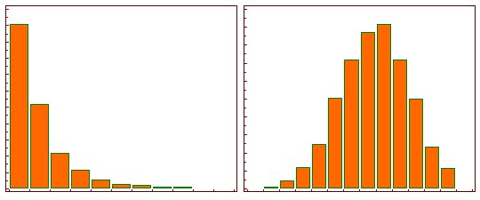
In symmetric distributions, one half of the distribution is a mirror image of the other half. Skewness is an asymmetry in the statistical distribution in which the curve appears distorted either to the left or to the right. A lot of real-world data forms a skewed distribution.

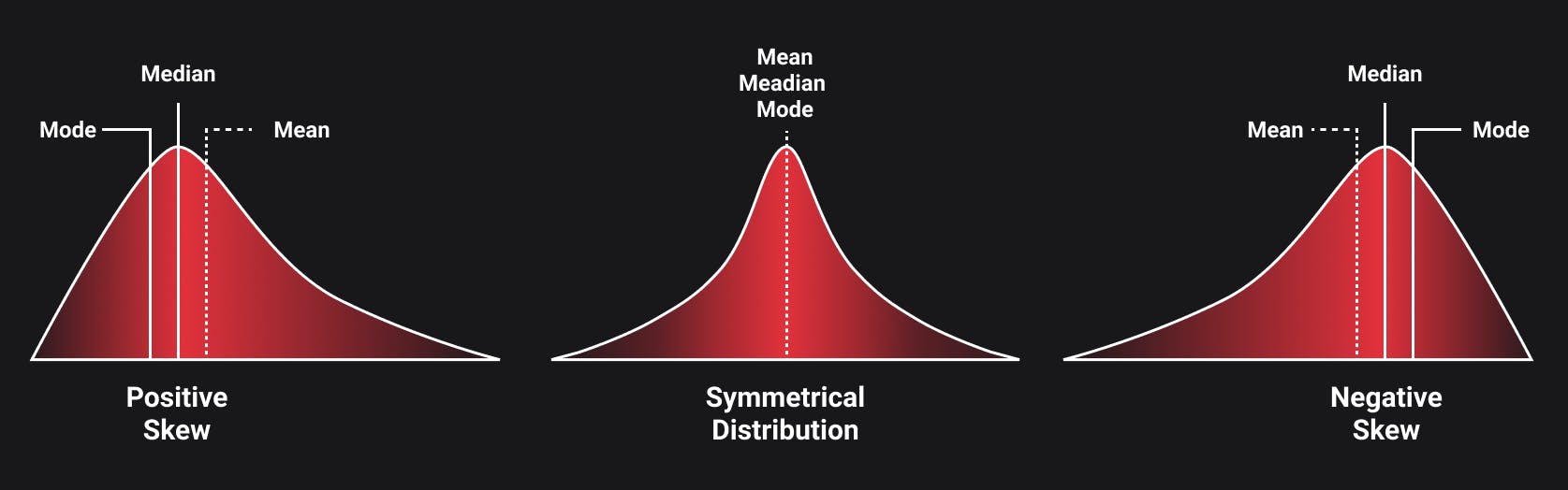
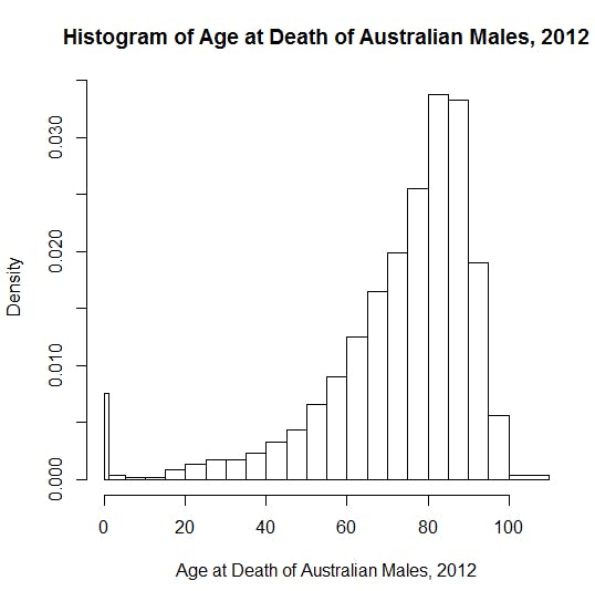
When a distribution is skewed to the left, the tail on the curve's left-hand side is longer than the tail on the right-hand side, and the mean is less than the mode. This situation is called negative skewness. The average human lifespan forms a negatively skewed distribution. This is because most people tend to die after reaching the mean age, and only a small number of people die too soon. If such data is plotted along a linear line, most of the values would be present on the right side, and only a few values would be present on the left side.

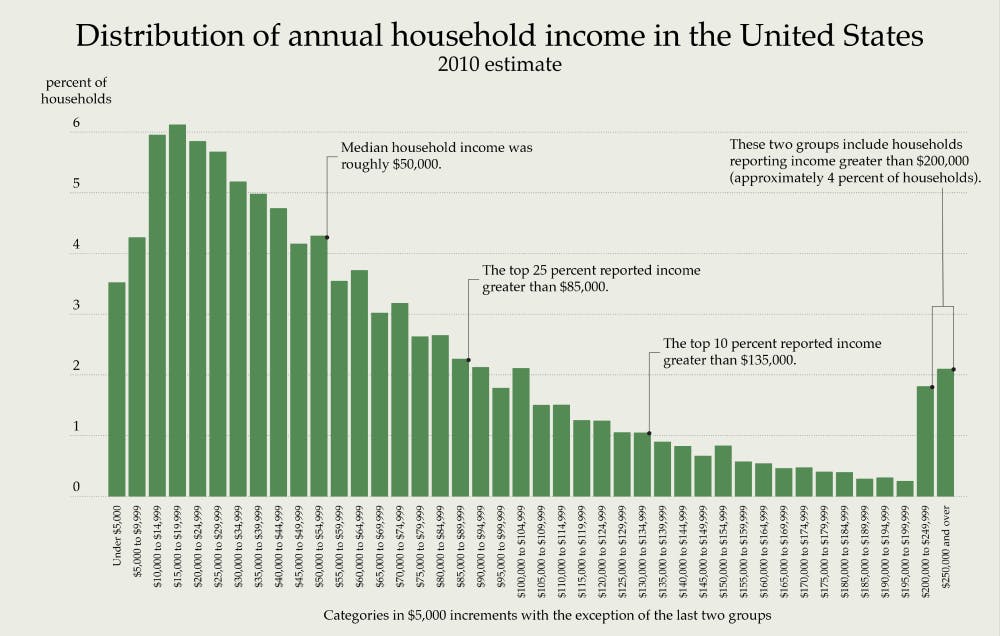
When a distribution is skewed to the right, the tail on the curve's right-hand side is longer than the tail on the left-hand side, and the mean is greater than the mode. This situation is called positive skewness. The income distribution of a state is an obvious example of a positively skewed distribution. A huge portion of the total population residing in a particular state tends to fall under the category of a low-income earning group, while only a few people fall under the high-income earning group.

When you are working with a symmetrical distribution for continuous data, the mean and median(sometimes even mode) are equal. In this case, the choice doesn't matter because all of them represent the relevant information. However, if you have a skewed distribution, the median is often the better measure of central tendency.

When working with skewed data, the tail region acts as an outlier for the statistical models and can be detrimental to their performance, especially regression-based models. There are some statistical models that are robust to outliers like tree-based models but skewed data limits our ability to try different models This creates a need for transforming skewed distribution into a more "normal" distribution, you do so by using log transformation.

Log transformation simply replaces each variable x with a log(x). The choice of the logarithm base depends on the purpose of statistical modeling but natural log is a good place to start.

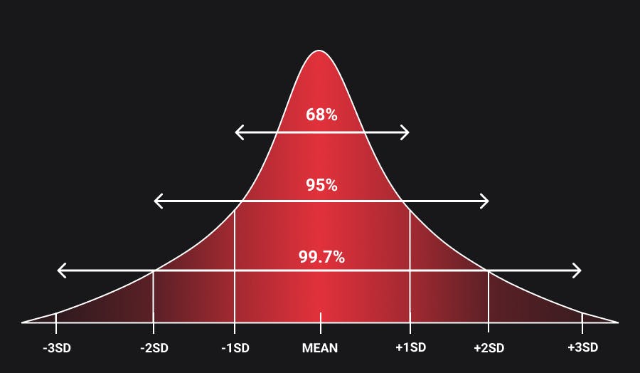
Empirical Rule

The empirical rule, also known as the three-sigma rule or 68-95-99.7 rule, states that for the normal distribution, nearly all of the data will fall within three ranges of standard deviations of a mean.

The empirical rule can be understood through the following:

• 68.3% of the data falls within the first standard deviation from the mean.
• 95.5% falls within two standard deviations.
• 99.7% falls within three standard deviations.

The empirical rule helps determine outcomes when not all the data is available. It allows us to gain insight into where the data will fall, once all of it is available.

It is also used to test how normal a data set is. If the data does not adhere to the empirical rule, then it is not considered a normal distribution and must be treated accordingly.

Standard Normal Distribution

A Standard Normal Distribution is a normal distribution that has a mean \(\mu\) equal to zero and standard deviation \(\sigma\) is equal to one. We can standardize any distribution using the Z-score formula. Z-score (also called a standard score) is a measure of how many standard deviations below or above the population mean a raw score is. Simply put, the z-score gives you an idea of how far from the mean a data point is.

\[ Z = \frac {x - \mu}{\sigma} \]

What's the need for this standardization?

Different distributions that are normal will have different means and standard deviations. To be able to find the probability of a given characteristic (say the height of students in a class) lying within a given interval, we have to integrate the density function within the limits given the \(\mu\) and \(\sigma\) of the distribution. For each study, we would have to follow a similar process which can be tedious. This is where standard normal distribution to our rescue. For the standard normal distribution the value of the parameters are known:(\(\mu = 0\), \(\sigma = 1\)). So for a standard normal distribution, we have the standard normal chart which shows us the area under the curve for all values between 0 to +-3 \(\sigma\). Standardization of a normal variate does not affect the characteristics of the distribution and hence we can use it to easily compute required probabilities.

TLDR: Using standardized normal distribution makes inferences and predictions much easier.

We're gonna stop here for now, in the second part we'll cover the remaining three distributions, and then go on to learn about sampling and hypothesis testing.