Demystifying Probability Distributions(Part

Continuing from where we left off in the previous part of the statistics series, let's talk about the remaining probability distributions, starting with the binomial distribution.

Binomial Distribution

Bernoulli Trial

Bernoulli trial is a random experiment that has exactly two possible outcomes and the probability of each outcome remains the same each time the experiment is conducted.

\[ P(X = x) = \begin{cases} p &\text{if } 1 \\ (1 - p) &\text{if } 0 \end{cases} \]

A coin flip is an example of an experiment with a binary outcome. Coin flips meet the other requirement as well — the outcome of each individual coin flip is independent of all the others. The outcomes of the experiment don’t need to be equally likely as they are with flips of a fair coin, the following things also meet the prerequisites of the Bernoulli trial:

The answer to a True or False question
Winning or losing a game of Blackjack
Attempting to convince visitors of a website to buy a product, the yes or no outcome is whether they make a purchase.

What is binomial distribution?

The binomial distribution is the probability distribution of a series of random Bernoulli trials that produce binary outcomes, each of these outcomes is independent of the rest.

A series of 5 coin flips is a straightforward example, using the formula mentioned below we can get the probabilities of getting 1, 2, 3, 4, or 5 heads.

\[ P(X) = \binom{n}{x}p^x(1-p)^{n-x} \]

Here

\(n\) is the total number of trials of an event.
\(x\) corresponds to the number of times an event should occur.
\(p\) is the probability that the event will occur.
\(1-p\) is the probability that the event will not occur.
\( \binom{n}{x}\) is the formula for all possible combinations,i.e., \( \frac{n!}{x!(n-x)!}\)

Let's use this to calculate the probability of getting 5 heads in 10 tosses, and verify the findings by simulating the experiment 10,000 times.

\[ P(X) = \binom{10}{5}\frac{1}{2}^5(1-\frac{1}{2})^{5} \]

\[ => .246 \]

import numpy as np

trials = 10000
n = 10
p = 0.5

prob_5 = sum([1 for i in np.random.binomial(n, p, size = trials) if i==5])/trials
print('The probability of 5 heads is: ' + str(prob_5))

The probability of 5 heads is: 0.242

But what if you wanted to plot the distribution of probabilities for all possible values of \(x\)?

import matplotlib.pyplot as plt
import seaborn as sns

# Number of trials
trials = 1000
# Number of independent experiments in each trial
n = 10
# Probability of success for each experiment
p = 0.5

# Function that runs our coin toss trials
def run_trials(trials, n, p):
    head = []
    for i in range(trials):
        toss = [np.random.random() for i in range (n) ]
        head.append (len ([i for i in toss if i>=0.50]))
    return head

heads = run_trials(trials, n, p)

# Ploting the results as a histogram
fig, ax = plt.subplots(figsize=(14,7))
ax = sns.distplot(heads, bins=11, label='simulation results')

ax.set_xlabel("Number of Heads",fontsize=16)
ax.set_ylabel("Frequency",fontsize=16)

# Ploting the actual/ideal binomial distribution
from scipy.stats import binom
x = range(0,11)
ax.plot(x, binom.pmf(x, n, p), 'ro', label='actual binomial distribution')
ax.vlines(x, 0, binom.pmf(x, n, p), colors='r', lw=5, alpha=0.5)
plt.legend()
plt.show()

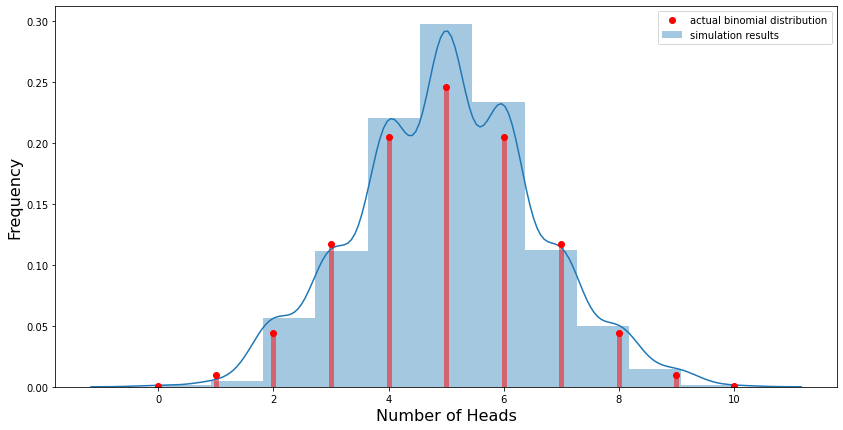
Does the shape of the plot remind you of normal distribution? Well, it should. This is because of the concept of Normal approximation. If n is large enough, a reasonable approximation to \(B(n, p)\) can be given by the normal distribution \(N(np, np(1-p)\). This can be seen visually in the Galton Board demonstration below.

Student's T Distribution

The Student's T distribution is bell-shaped & symmetric, similar to the normal distribution, but has more massive tails. It is used in place of the normal distribution when we have small samples (n<30). T distribution starts resembling normal distribution when the sample size increases.

\[ f(t) = \frac {\varGamma \frac{\nu + 1}{2}}{\sqrt {\nu \pi} \varGamma \frac{\nu}{2}}(1 + \frac{t^2}{\nu})^\dfrac{\nu + 1}{2} \]

Don't worry about this formula, you'll probably never need it but if you want to, you can learn more about what it means here.

What's the need for Student's T distribution?

Statistical normality is overused. It‘s not as common and only really occurs in the theoretical ‘limits’. To garner normality, you need to have a substantial well-behaved independent dataset but for most cases, small sample sizes and independence are usually what we have. We tend to have sub-optimal data that we manipulate to look normal but in fact, those anomalies in the extremes are telling you something is up.

Lots of things are ‘approximately’ normal. That’s where the danger is.

A lot of the unlikely events are actually more likely than we expect and this is not because of skewness, but because we’re modeling the data wrong. Let's take an over-exaggerated example of ambient temperature forecast over a 100 year period. Is 100 years of data enough to assume normality? Yes? No! The world has been around for millions and millions of years, 100 years is insignificant. However, to reduce computational complexity and make things simpler we choose a small portion of the total data in most cases. By doing so we underestimating the tails.

Therefore, it is important to know what you don’t know and the distribution that you’re using for your inferences. The normal distribution is used for inferences mainly because it offers a tidy closed-form solution but in reality, the difficulties in solving harder distributions are why, at times, they make better predictions.

Let's say we have a random variable with a mean μ and a variance σ², derived from a normal distribution. Then we know that if we find a sample estimate of the mean (say μ⁰), then the following variable z = [μ⁰-μ] / σ is a normal distribution, but, it now has a mean of 0 and a variance of 1. We’ve normalized the variable, or, we’ve standardized it.

However, imagine we have a relatively small sample size (say n < 30) which is part of a greater population. Then our estimate of mean (μ) will remain the same, however, our estimate of standard deviation, our sample standard deviation, has a denominator of n-1 (Bessel's correction).

Because of this, our attempt to normalize our random variable has not resulted in a standard normal, but rather has resulted in a variable with a different distribution, namely: a Student-t Distribution of the form:

\[ t = \frac{|\bar{x} - \mu|} {\Large {\frac {s}{\sqrt{n}}}} \]

\(\bar{x}\) is the sample mean, μ is the estimate of the population mean, s is the standard error, and n is the number of samples.

This is significant to note because it tells us that even though something may be normally distributed, in small sample sizes, the dynamics of sampling from this distribution completely change, which is largely being characterized by Bessel’s correction.

Poisson Distribution

The Poisson distribution gives us the probability of certain events happening when we know how often the events have occurred. Simply put, the Poisson Distribution function gives the probability of observing \(k\) events in a given length of the time period and the average events per time period. \[ P(\text{k events in interval}) = e ^ {-\frac{event}{time} time \kern{1px} period} \frac { {\frac{event}{time} time \kern{1px} period} ^ k} {k!} \] The \(\frac{event}{time} * \text{time period}\) is usually simplified into a single parameter, \(λ\), lambda, the rate parameter. Lambda can be thought of as the expected number of events in the interval. \[ P(\text{k events in interval}) = \frac {e ^ {-\lambda} \lambda ^ k} {k!} \]

here:

\(k\) is the number of occurrences
\(e\) is Euler's number (e = 2.71828...)
\(λ\) is the rate parameter.

Let's use an example to make sense of all this. Suppose that in a coffee shop, the average number of customers per hour is 4. We can use the Poisson distribution formula to calculate the probability of getting k number of customers in the shop.

from scipy.stats import poisson 
import numpy as np 
import matplotlib.pyplot as plt 

no_of_customers = np.arange(0, 15, 1) 
lamda = 4
probs = poisson.pmf(no_of_customers, lamda) 

plt.figure(figsize=(15, 10))
plt.bar(no_of_customers, probs) 
plt.show()

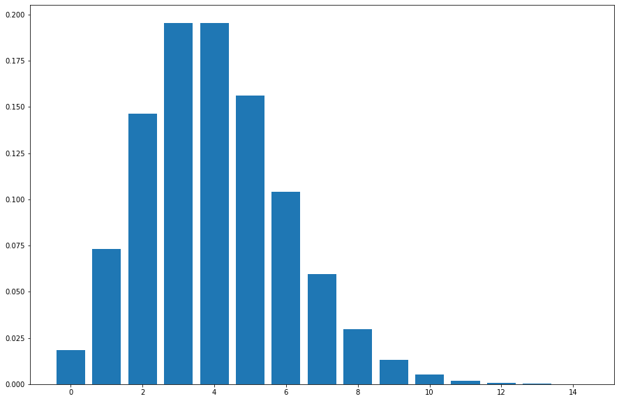
What about the probability of seeing less than let's say, 7 customers? We can simply get that by integrating the Poisson curve for the limits of 0 -> 7, or simply add the probabilities of all values of k < 7.

print(f"Probability of seeing less than 7 customers is {np.around(sum(probs[:8]),3)}")

Probability of seeing less than 7 customers is 0.949

Conditions for Poisson Distribution:

The events can occur independently.
An event can occur any number of times.
The rate of occurrence is constant; i.e., the rate does not change based on time.

As the rate parameter, λ, changes so does the probability of seeing different numbers of events in one interval. The below graph is the probability mass function of the Poisson distribution showing the probability of a number of events occurring in an interval with different rate parameters.

from scipy.stats import poisson 
import numpy as np 
import matplotlib.pyplot as plt 

x = np.arange(0, 50, 1) 
plt.figure(figsize=(15, 10))
# poisson distribution data for y-axis 
y1 = poisson.pmf(x, mu=10) 
y2 = poisson.pmf(x, mu=15)
y3 = poisson.pmf(x, mu=25)
y4 = poisson.pmf(x, mu=30)

plt.plot(x, y1, marker='o', label = "lambda = 10") 
plt.plot(x, y2, marker='o', color = "red", label = "lambda = 15" )
plt.plot(x, y3, marker='o', color = "green", label = "lambda = 25")
plt.plot(x, y4, marker='o', color = "magenta", label = "lambda = 30")

plt.legend()
plt.show()

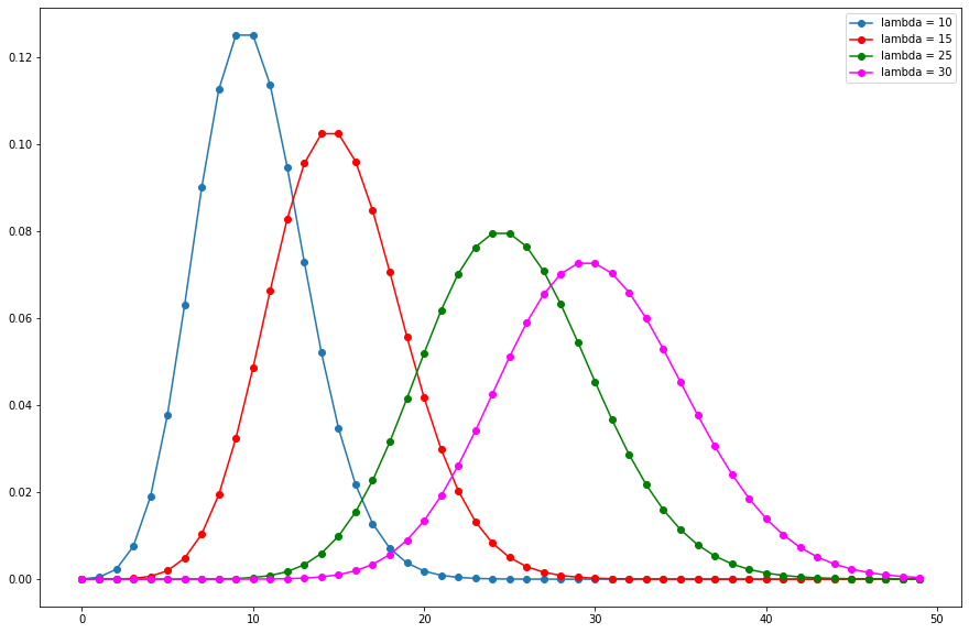
The most likely number of events in the interval for each curve is the rate parameter. This makes sense because the rate parameter is the expected number of events in the interval and therefore when it’s an integer, the rate parameter will be the number of events with the greatest probability.

With that we're done with the probability distributions, in the next article we'll learn about sampling and the central limit theorem. 👋

Gradient Ascent