

In the first article of the series, we discussed the fundamentals of statistics, and how statistical analysis is used to find patterns and make predictions. Well, the statistical inferences are based on probability. So understanding probability and its characteristics are essential to effectively tackle machine learning problems. That's what we are going to cover in this article.
In this article, we will go through the Frequentist interpretation of probability as it is easier to understand from a beginner’s point of view. You can read about the other interpretations of probability here.
The most important questions of life are indeed, for the most part, really only problems of probability. — Pierre-Simon Laplace
Events
Events are one of the most basic concepts in statistics, simply put they are the results of experiments or processes. An event can be certain, impossible, or random.
An experiment is defined as the execution of certain actions within a set of conditions.
An event is said to be certain if it will occur at every performance of the experiment. Take, for instance, the event of getting a number less than 7 when throwing a die. On the other hand, impossible events are events that will not occur as a result of the experiment. For example, the event of getting a 7 when throwing a die.
And lastly, an event is called a random event if it may or may not occur as a result of the experiment. These are outcomes of random factors whose influence cannot be predicted accurately if they can be predicted at all. Let’s take the case of a dice roll, the experiment is influenced by random factors like the shape and physical characteristics of the dice, the strength & method of the throw, and environmental factors such as air resistance. Accurately predicting factors like these is basically impossible.
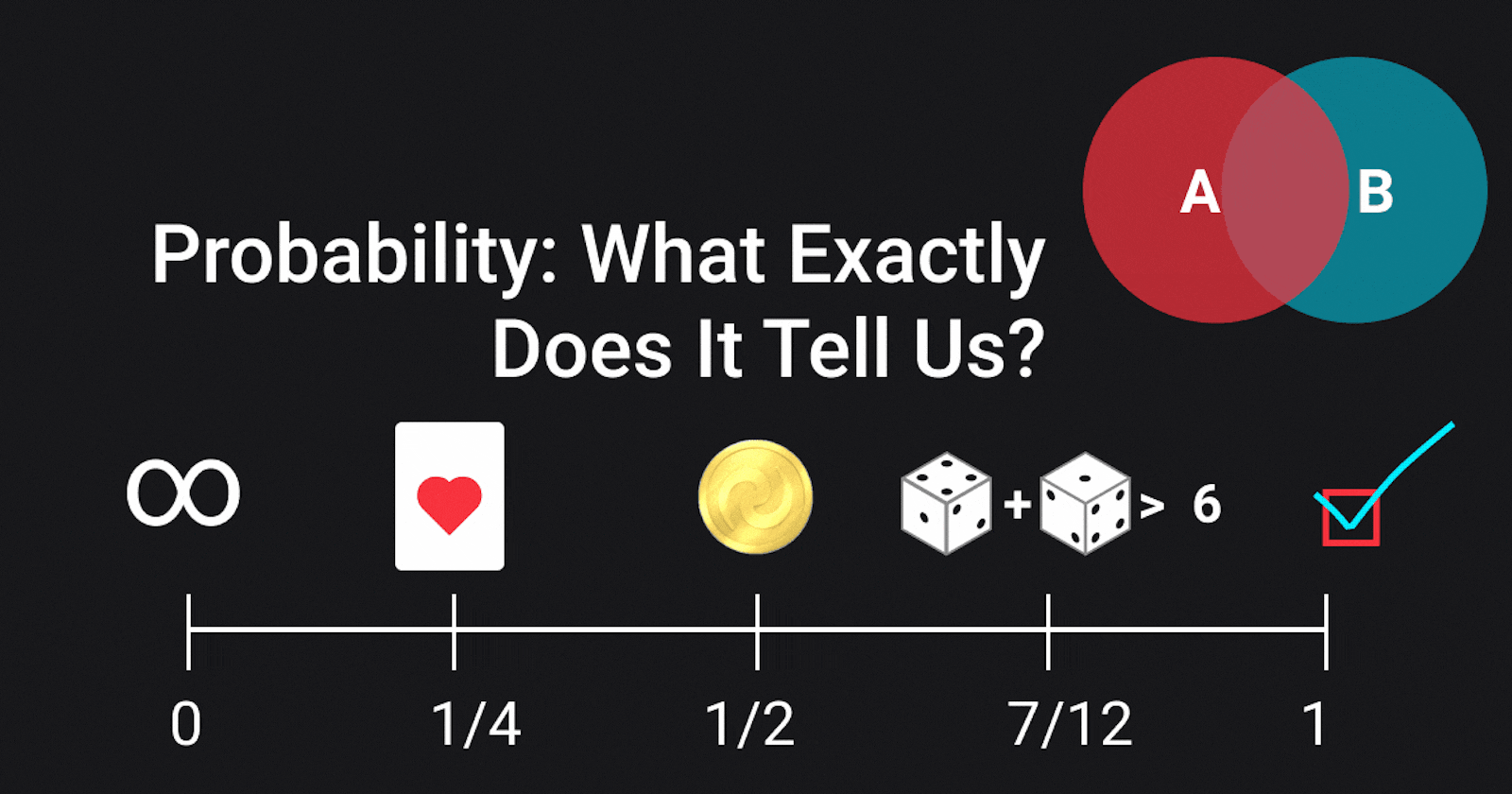
What Is Probability?
Let’s go more in-depth in analyzing a random event, for instance, a fair coin toss. A fair experiment is one in which all outcomes are equally likely. There are two possible outcomes of a coin toss — heads or tails. The outcome of the flip is considered random because the observer cannot analyze and account for all the factors that influence the result. Now, if I were to ask you what is the probability of the toss resulting in heads, you would probably say ½, but why?
Let’s name the event that came up as head A, and let’s say the coin is tossed n times. Then the probability of event A can be defined as its frequency in a long series of experiments, or:
Probability of event A = Number of ways A can happen / Total number of outcomes
Let’s take another example, a deck of playing cards. There are four Aces in a deck, what is the probability of drawing an Ace from the deck?
Total number of outcomes: 52 (total number of cards)
Number of ways the event can happen: 4
So the probability becomes 4/52, or 1/13
Now you might say that the chances of drawing an ace or getting tails don’t always match these expectations. And you have good reasons to say so. If we were to conduct a series of tests, the probability of an event A would fluctuate around a constant value P(A) for large n. This is the value we call the probability of event A. It basically means that if we were to carry out the experiment for a sufficiently large n, ideally infinite, we would get the event A P(A) x n times.
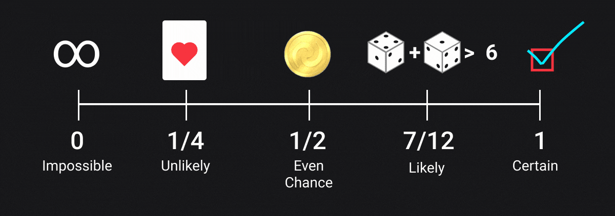
The probability of all events lies in the range [0, 1], the probability of 0 indicates impossibility, and 1 indicates certainty.
Types of Events
Independent & Dependent Events
Two events A and B are said to be independent events if the occurrence of one of them does not influence the probability of seeing the other. For example, having the information that a coss toss resulted in heads on the first toss doesn’t provide us with any useful information for predicting what the outcome of the second toss will be. The probability of a head or a tail remains 1/2 regardless of the outcome of the previous toss. The probabilities of independent events are multiplied to get the total probability of occurrence of all of them.
Let’s illustrate this with an example: What is the probability of getting tails three times in a row?
Firstly, let’s calculate this using our original formula of probability.
Possible outcomes of 3 coin tosses: HHH, HHT, HTH, THH, TTT, TTH, THT, HTT
Number of ways the event can happen: 1
Total number of outcomes: 8
The probability is ⅛, but we know that the outcomes of consecutive coin tosses are independent so we can simply multiply them to get the probability of TTT: P(T) x P(T) x P(T) = ½ x ½ x ½ = ⅛
On the other hand, if the occurrence of one event changes the probability of the other, the events are said to be dependent. Knowing that the first card drawn from a deck is a Jack changes the probability of drawing another Jack from 4/52 to 3/51. This is precisely why counting cards is a thing.
Disjoint & Overlapping Events
Disjoint events, also known as mutually exclusive events, cannot happen at the same time. For example, the outcome of a coin toss cannot be head and tail at the same time. On the flip side, the events that are not disjoin can happen at the same time, and can thus overlap. To avoid double-counting in such cases the probability of overlapping should be subtracted from total probability.
Take for instance the probability of drawing a Queen or Spades card from a deck. There are several ways this can happen: 4 (because there are 4 Queens) and 13 (there are 13 cards of the suit Spade). However, 1 card overlaps between them - the Queen of Spades.
So P(Queen or Spades) = P(Queen) + P(Spades) - P(Queen of Spades) = 4/52 + 13/52 -1/52 = 4/13
Types of Probabilities
Joint Probability
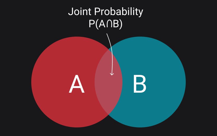
The joint probability for two non-disjoint events A and B is the probability of them occurring at the same time. The joint probability is obtained by multiplying the probabilities of the two events. For example, the total probability of drawing a black Ace card is P(Ace ∩ black) = 2/52 = 1/26. This can also be calculated using the formula: P(Ace ∩ black) = P(Ace) x P(black) = 4/52 x 26/52 = 1/26.
The symbol “∩” in joint probability indicates an intersection, the probability of two events A and event B is the same as the intersection of A and B sets. This can be best visualized with the help of Venn diagrams.
Marginal Probability
Marginal probability is the probability of an event occurring irrespective of what may or may not have happened. It can be thought of as unconditional probability as is not affected by other events.
Conditional Probability
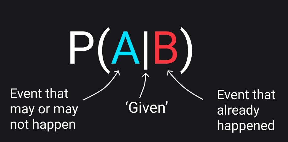
P(A|B), which means the probability of event A given that event B has occurred, or simply given B. It is given by
P(A|B) = P(A ∩ B) / P(B)
Let’s illustrate this using an example: In a class of 100 students, 23 students like to play both football and basketball and 45 of them like to play basketball. What is the probability that a student who likes playing basketball also likes football?
P(football | basketball) = P(football ∩ basketball) / P(basketball)
P(football | basketball) = .23/.45 = .51
That’s it for this one, if some of these concepts are still a bit blurry, don’t worry. It will start to make more sense when we talk about these in the context of things like the Bayes theorem and probability distributions in later blogs.