If you come from a statistical or data science background you must be familiar with the importance of data cleaning and feature engineering. Well, what's the computer vision equivalent of the two? Image transformations. From removing noise and fixing perspective skews to using image augmentation to make the most out of a limited dataset, image transformations are an essential part of computer vision pipelines.

Simply put transformations are geometric distortions enacted on an image, these distortions can be simple things like resizing, rotation, translation. However, there are also some more complex distortions such as warp transformation which is used to correct perspective issues arising from the point of view an image was captured from. Transformations are classified into two broad categories in computer vision - Affine and Non-Affine Transformations

Affine and Non-Affine Transformations

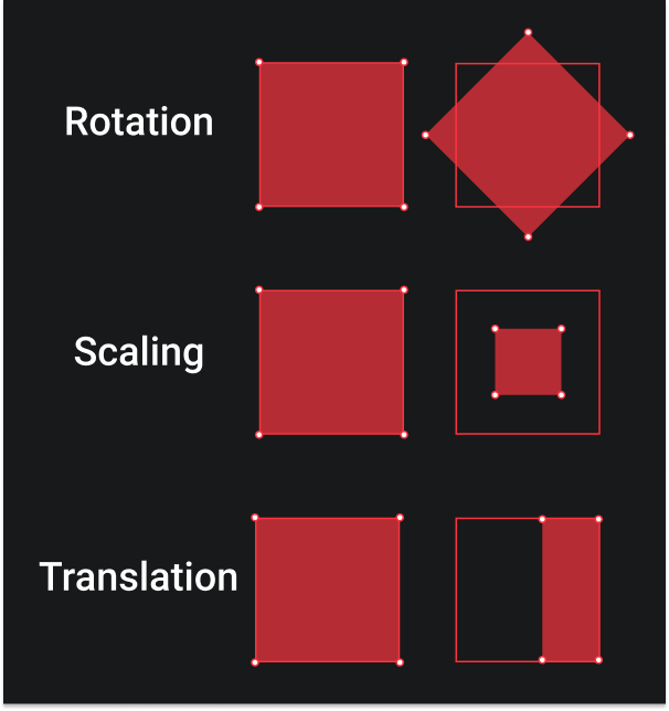
Affine transformations include things such as scaling, rotation, and translation. The key point to remember is that the lines that were parallel in the original image remain parallel in the transformed images. So whether you scale an image, rotate, or scale it, the parallelism between lines is maintained.

This is not the case in non-affine transformations which are also known as projective transformations. They do, however, preserves collinearity. What this means is that points that lie on a line before the transformation will continue to do so in the transformed image.

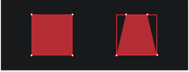
Non-affine transformations are very common in computer vision, and they originate from different camera angles. Take for instance the illustration above, on the left, you're looking at the square from a top-down perspective. As you slowly start to move the camera downwards your view will become skewed. The points that are further from you will start to appear closer together than the points closest to you.

Now let's actually see how we can apply these transformations in OpenCV.

Translation

Translations are very simple, it's just basically moving an image in one direction. This can be up, down, or even diagonally. To perform translations we use OpenCV's cv2.warpAffine function which requires a translation matrix \( T \). Let's quickly understand the translation matrix without getting into too much geometry, it takes the following form:

\[ T = \begin{equation} \begin{bmatrix} 1 & 0 & T_x \\ 0 & 1 & T_y \\ \end{bmatrix} \end{equation} \]

Here

• \( T_x \) : represents shift along x-axis
• \( T_y \) : represents shift along y-axis

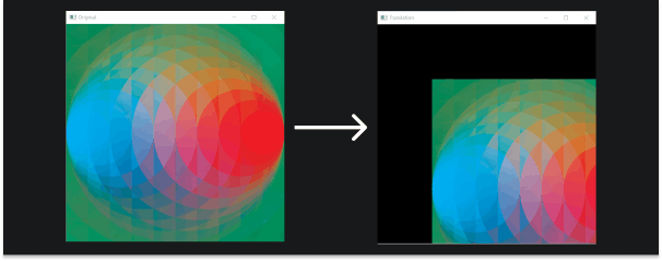
Now let's actually apply the transformation to an image. We are going to translate an image down diagonally, we'll do so by shifting it a quarter of its height and width.

import cv2
import numpy as np

image = cv2.imread('images/ripple.jpg')
height, width = image.shape[:2]
quarter_height, quarter_width = height/4, width/4

# making the translation matrix
T = np.float32([[1, 0, quarter_width], [0, 1,quarter_height]])

# warpAffine takes as argument the image, translation matrix T
# and the dimensions of the output image
img_translation = cv2.warpAffine(image, T, (width, height))
cv2.imshow('Original', image)
cv2.imshow('Translation', img_translation)
cv2.waitKey()
cv2.destroyAllWindows()

Rotation

Rotations are also pretty simple as well but there are some quirks. Similar to our translation transformation, rotation is done using the cv2.warpAffine function but instead of passing in a translation matrix \( T \), we pass a rotation matrix \( M \) that can be easily created using cv2.getRotationMatrix2D function. \[ M = \begin{equation} \begin{bmatrix} \cos\theta & - \sin\theta \\ \sin\theta & \cos\theta \\ \end{bmatrix} \end{equation} \]

Here \( \theta \) is the angle of rotation.

cv2.getRotationMatrix2D takes three arguments a tuple representing the coordinates of the pivot point (x,y), the angle of rotation \( \theta \) , a float scale value. "What's the need for a scale value?" That's what you're thinking, right? Well, let's try rotating our image by 45 degrees about its center and see what happens.

image = cv2.imread('images/ripple.jpg')
height, width = image.shape[:2]

# dividing the dimensions by two to rototate the image around its centre
rotation_matrix = cv2.getRotationMatrix2D((width/2, height/2), 45, 1)
rotated_image = cv2.warpAffine(image, rotation_matrix, (width, height))

cv2.imshow('Rotated Image', rotated_image)
cv2.waitKey()
cv2.destroyAllWindows()

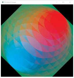
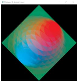
Notice the black space around it? and how parts of the image are cropped out. This is further exaggerated when working with portrait or landscape images. So if we want to use the whole image after rotating it regardless of its initial size and orientation, scaling it down makes sense.

rotation_matrix = cv2.getRotationMatrix2D((width/2, height/2), 45, .7)
rotated_image = cv2.warpAffine(image, rotation_matrix, (width, height))

cv2.imshow('Rotated & Scaled Image', rotated_image)
cv2.waitKey()
cv2.destroyAllWindows()

If you only want to rotate the image by 90 degrees without worrying about the size and orientation of the image you can use the cv2.transpose function.

rotated_image = cv2.transpose(image)
cv2.imshow('Rotated Image - Transpose', rotated_image)

Another handy function worth remembering is the cv2.flip function that flips the image based on the axis argument.

# Horizontal Flip
flipped_h = cv2.flip(image, 1)

# Vertical Flip
flipped_v = cv2.flip(image, 0)

Resizing & Interpolation

If you have read the first article of the series, you already have a decent understanding of how resizing works in OpenCV. To recap, you can use the cv2.resize function to resize an image. There are two ways of selecting the target size, you can either pass the desired dimensions as a tuple

resized_images = cv2.resize(image, (256, 256))

or scale it using the scaling factors fx and fy

resized_image = cv2.resize(image, None, fx=.5, fy=.5)

Resizing is a simple transformation, for the most part, the only nuanced thing is the choice of interpolation method. Interpolation is an estimation method that creates new data points between a range of known data points. In the context of images and resizing, interpolation is used to create new data points when "zooming in" or expanding the image, and deciding which points to exclude when "zooming out" or shrinking the image. There are a bunch of interpolation methods supported by OpenCV but comparing them is beyond the scope of this article, you can find a good comparison here.

Here's a list of all the methods and general intuition regarding when to use what:

• cv2.INTER_AREA - Good for shrinking or downsampling
• cv2.INTER_NEAREST - Fastest
• cv2.INTER_LINEAR - Good for zooming or upsampling (default)
• cv2.INTER_CUBIC - Better
• cv2.INTER_LANCZOS4 - Best

You can select the interpolation method by passing the respective flag to the interpolation argument.

img_scaled = cv2.resize(image, None, fx=2, fy=2, interpolation = cv2.INTER_CUBIC)

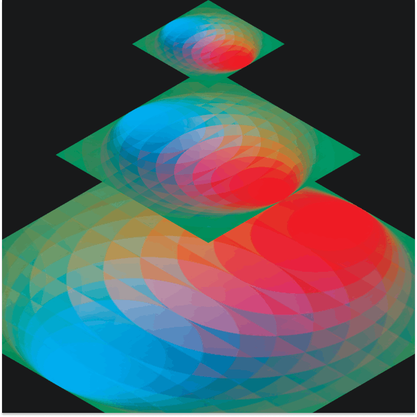
Image Pyramids

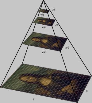
Image pyramids are a multi-scale representation of an image, they allow us to quickly scale images. Scaling down reduces the height and width of the new image by half, and similarly, scaling up increases the dimensions by a factor of 2. This is extremely useful when working with something like object detectors that scale images each time they look for an object.

You can use the and to quickly scale up and scale down images, respectively.

image = cv2.imread('images/ripple.jpg')

smaller = cv2.pyrDown(image)
larger = cv2.pyrUp(image)

cv2.imshow('Original', image )
cv2.imshow('Smaller ', smaller )
cv2.imshow('Larger ', larger )

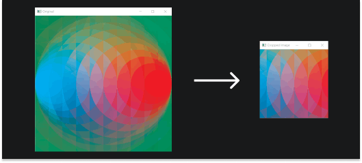
Cropping

Cropping images is fairly straightforward and you have probably done it before. It is useful for extracting regions of interest from images. Images are stored as arrays so cropping images is just a matter of slicing the arrays appropriately.

image = cv2.imread('images/ripple.jpg')
height, width = image.shape[:2]

# let's get the starting pixel coordiantes (top  left of cropping area)
start_row, start_col = int(height * .25), int(width * .25)

# now the ending pixel coordinates (bottom right)
end_row, end_col = int(height * .75), int(width * .75)

# Simply use array indexing to crop out the area we desire
cropped = image[start_row:end_row , start_col:end_col]

cv2.imshow("Original Image", image)
cv2.imshow("Cropped Image", cropped)

Arithmetic & Bitwise Operations

Arithmetic operations allow us to directly add or subtract the color intensity. It calculates the per-element operation of two arrays. The overall effect is an increase or decrease in brightness.

image = cv2.imread('images/ripple.jpg')

# creating a matrix of ones, then multiply it by a scaler of 100 
# This gives a matrix with the same dimensions 
# as our image with all values being 100
X = np.ones(image.shape, dtype = "uint8") * 100

# We use this to add this matrix X, to our image
# Notice the increase in brightness
added = cv2.add(image, X)
cv2.imshow("Added", added)

# Likewise we can also subtract
# Notice the decrease in brightness
subtracted = cv2.subtract(image, X)
cv2.imshow("Subtracted", subtracted)

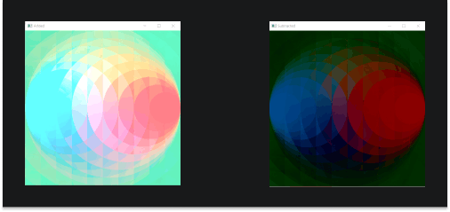
One thing to note when adding or subtracting from an image is that you can't exceed 255 or go below 0. For instance, if the value of a pixel becomes 256 after addition it will revert to 255, and if the value of a pixel becomes -2, it will revert to 0.

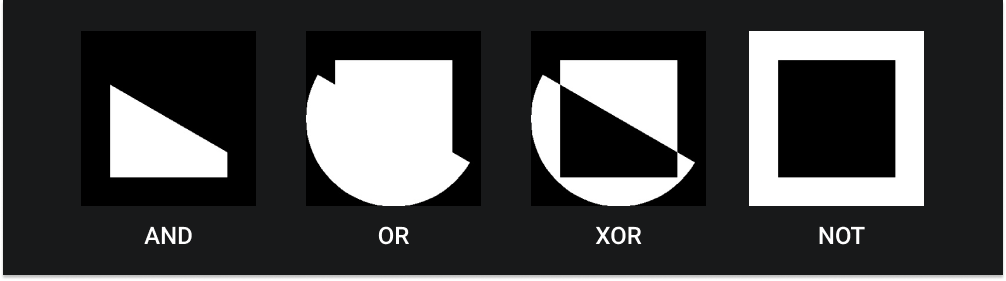
Bitwise operations perform logical operations like AND, OR, NOT & XOR on two images. They are used with masks as we saw in the first article of the series.

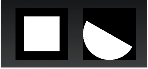
Let's create some shapes to demonstrate how these work.

# making a sqare
square = np.zeros((300, 300), np.uint8)
cv2.rectangle(square, (50, 50), (250, 250), 255, -2)
cv2.imshow("Square", square)

# making a ellipse
ellipse = np.zeros((300, 300), np.uint8)
cv2.ellipse(ellipse, (150, 150), (150, 150), 30, 0, 180, 255, -1)
cv2.imshow("Ellipse", ellipse)

Now let's perform some logical operations using these.

# shows only where the shapes intersect
and = cv2.bitwise_and(square, ellipse)
cv2.imshow("AND", and)

# shows where either square or ellipse is 
bitwiseOr = cv2.bitwise_or(square, ellipse)
cv2.imshow("OR", bitwiseOr)

# shows where either shape exist by itself
bitwiseXor = cv2.bitwise_xor(square, ellipse)
cv2.imshow("XOR", bitwiseXor)

# shows everything that isn't part of the square
bitwiseNot_sq = cv2.bitwise_not(square)
cv2.imshow("NOT - square", bitwiseNot_sq)

Blurring, Convolution & Sharpening

Convolution

Convolution is a mathematical operation performed on two functions (f and g) producing a third function (f \( \otimes \) g) which is a modified version of one of the original functions. This new function expresses how the shape of one is modified by the other.

In the context of computer vision, convolution is the process of adding pixel values of the image to their local neighbors, weighted by a kernel. The kernel is just a small matrix, the size and values change depending on the type of image processing operation we want to apply.

Despite being denoted by \( \otimes \), the matrix operation being performed is not the normal matrix multiplication.

\[ \left (
\begin{equation} \begin{bmatrix} 1 & 2 & 3 \\ 4 & 5 & 6 \\ 7 & 8 & 9 \\ \end{bmatrix} \otimes \begin{bmatrix} a & b & c \\ d & e & f \\ g & h & i \\ \end{bmatrix} \end{equation} \right ) [2,2] = (a.9) + (b.8) + (c.7) + (d.6) + (e.5) + (f.4) + (g.3) + (h.2) + (i.1) \]

Blurring

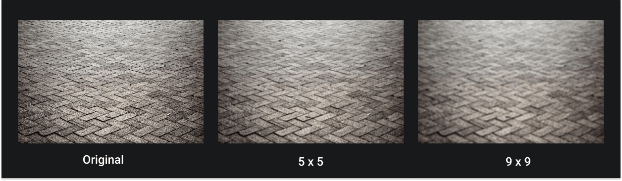
As you may have guessed it blurring is the operation where we average the pixels within a region. The blurring operation blends the edges in the images and makes them less noticeable.

The following is a 5 x 5 kernel used for averageblurring. We multiply it by 1/25 to normalize i.e. sum to 1, otherwise, the intensity of the image would increase.

\[ Kernel = \frac{1}{25} \begin{equation} \begin{bmatrix} 1 & 1 & 1 & 1 & 1 \\ 1 & 1 & 1 & 1 & 1 \\ 1 & 1 & 1 & 1 & 1 \\ 1 & 1 & 1 & 1 & 1 \\ 1 & 1 & 1 & 1 & 1 \\ \end{bmatrix} \end{equation} \]

We can apply any kernel on an image using the cv2.filter2D function, let's apply a 5 x 5 and 9 x 9 kernel on an image.

image = cv2.imread('images/pavement.jpeg')

# creating our 5 x 5 kernel
kernel_5x5 = np.ones((5, 5), np.float32) / 25

# use the cv2.fitler2D to conovlve the kernal with an image 
blurred_5x5 = cv2.filter2D(image, -1, kernel_5x5)
cv2.imshow('5x5 Kernel Blurring', blurred_5x5)

# creating our 9 x 9 kernel
kernel_9x9 = np.ones((9, 9), np.float32) / 81
blurred_9x9 = cv2.filter2D(image, -1, kernel_9x9)
cv2.imshow('9x9 Kernel Blurring', blurred_9x9)
`

Here's an awesome animation illustrating exactly how this convolution blurring process happens (source).

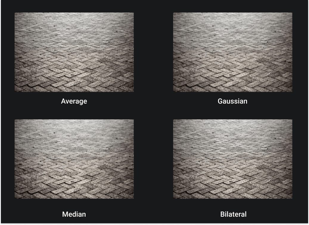
Commonly used blurring methods and what they do:

• cv2.blur – Averages values over a specified window like the ones we implemented above
• cv2.GaussianBlur – Similar to average blurring but uses a Gaussian window (more emphasis on points around the center) \[ Gaussian Kernel = \frac{1}{273} \begin{equation} \begin{bmatrix} 1 & 4 & 7 & 4 & 1 \\ 4 & 16 & 26 & 16 & 4 \\ 7 & 26 & 41 & 26 & 7 \\ 4 & 16 & 26 & 16 & 4 \\ 1 & 4 & 7 & 4 & 1 \\ \end{bmatrix} \end{equation} \]
• cv2.medianBlur – Uses median of all elements in the window
• cv2.bilateralFilter – It blurs the image while keeping edges sharp. It also uses a Gaussian filter, but adds one more Gaussian filter that is a function of pixel difference. This pixel difference function makes sure only those pixels with similar intensity to the central pixel are considered for blurring. This helps preserve the edges since pixels at edges will have large intensity variation. It highly effective for removing noise.

blur = cv2.blur(image, (3,3))
cv2.imshow('Averaging', blur)

# Instead of box filter, gaussian kernel
Gaussian = cv2.GaussianBlur(image, (7,7), 0)
cv2.imshow('Gaussian Blurring', Gaussian)

# Takes median of all the pixels under kernel area and central 
# element is replaced with this median value
median = cv2.medianBlur(image, 5)
cv2.imshow('Median Blurring', median)

# Bilateral is very effective in noise removal while keeping edges sharp
bilateral = cv2.bilateralFilter(image, 9, 75, 75)
cv2.imshow('bilateral Blurring', bilateral)

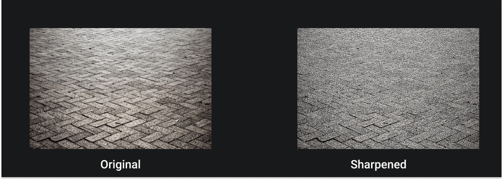
Sharpening

Sharpening is the opposite of blurring, it strengthens or emphasizes the edges in an image. In the case of sharpening, our kernel matrix will usually sum to one, so there is no need to normalize.

\[ Kernel = \frac{1}{25} \begin{equation} \begin{bmatrix} -1 & -1 & -1 \\ -1 & 9 & -1 \\ -1 & -1 & -1 \\ \end{bmatrix} \end{equation} \]

kernel_sharpening = np.array([[-1,-1,-1], 
                              [-1,9,-1], 
                              [-1,-1,-1]])

# applying the sharpening kernel to the image
sharpened = cv2.filter2D(image, -1, kernel_sharpening)
cv2.imshow('Image Sharpening', sharpened)

Perspective Transformation

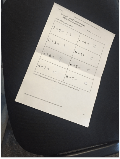
Perspective transformation enables use to extrapolate what an image would look like from a different camera angle. Consider the image above, it is a warped perspective of a perfectly rectangular piece of A4 paper as viewed from an angle. We can get the top-down perspective of this by using the cv2.warpPerspective function. The cv2.warpPerspective function applies a Perspective Transformation matrix, \( M \). OpenCV provides a method cv2.getPerspectiveTransform that generates this \( M \) matrix for us, it takes as an argument the two sets of coordinates. Firstly, the four corners of the object or region of interest and four corners of what we want the object/region to occupy.

It's important to remember that the second set of coordinates should correspond to sides that have a ratio similar to the ratio of dimensions of the object in real life. For example, an A4 sheet of paper has the ratio of 1:1.41, so we can use any set of coordinates as long the lengths of the sides have the ratio of 1:1.41. It's not that the transform won't work, just that it won't come out as nice. The whole point of the perspective transform is to fix skewed images, if the ratio is wrong we will just transform one skewed image into another.

image = cv2.imread('images/scan.jpg')

# cordinates of the 4 corners of the original image
points_A = np.float32([[320,15], [700,215], [85,610], [530,780]])

# cordinates of the 4 corners of the desired output
# We use the ratio of an A4 Paper 1 : 1.41
points_B = np.float32([[0,0], [420,0], [0,594], [420,594]])

# using the two sets of four points to compute 
# the Perspective Transformation matrix, M    
M = cv2.getPerspectiveTransform(points_A, points_B)

# warpPerspective also takes as argument 
# the final size of the image
warped = cv2.warpPerspective(image, M, (420,594))
cv2.imshow('warpPerspective', warped)

Pretty neat! Right?

That's it for now folks! In the next article, we will take a deeper dive into thresholding, learn about edge & contour detection. We will then use what we have learned so far to automate this process further to create our own scanner application. See ya!