
The very basic unit of input for any computer vision task is images, this can be diagnostic scans for medical use cases or individual video frames for surveillance and tracking models. In this article, we'll see how images are stored digitally, explore the two most common color models. All whilst familiarizing ourselves with the basics of OpenCV! And finding Nemo, at the end of the article we'll devise a mask that finds clownfish in images.
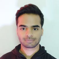
So what exactly constitutes an image? The individual pixels, obviously 😜. Digitally, each pixel is represented by a tuple or set of three values that represent its color in terms of the primitive colors- red, green and blue. These pixel tuples are stored in a two-dimensional array that has the same dimensions as the image. This makes the dimensions of the image array MxNx3 where M and N are the image dimensions. If an image array was flattened out and this is what it would look like:
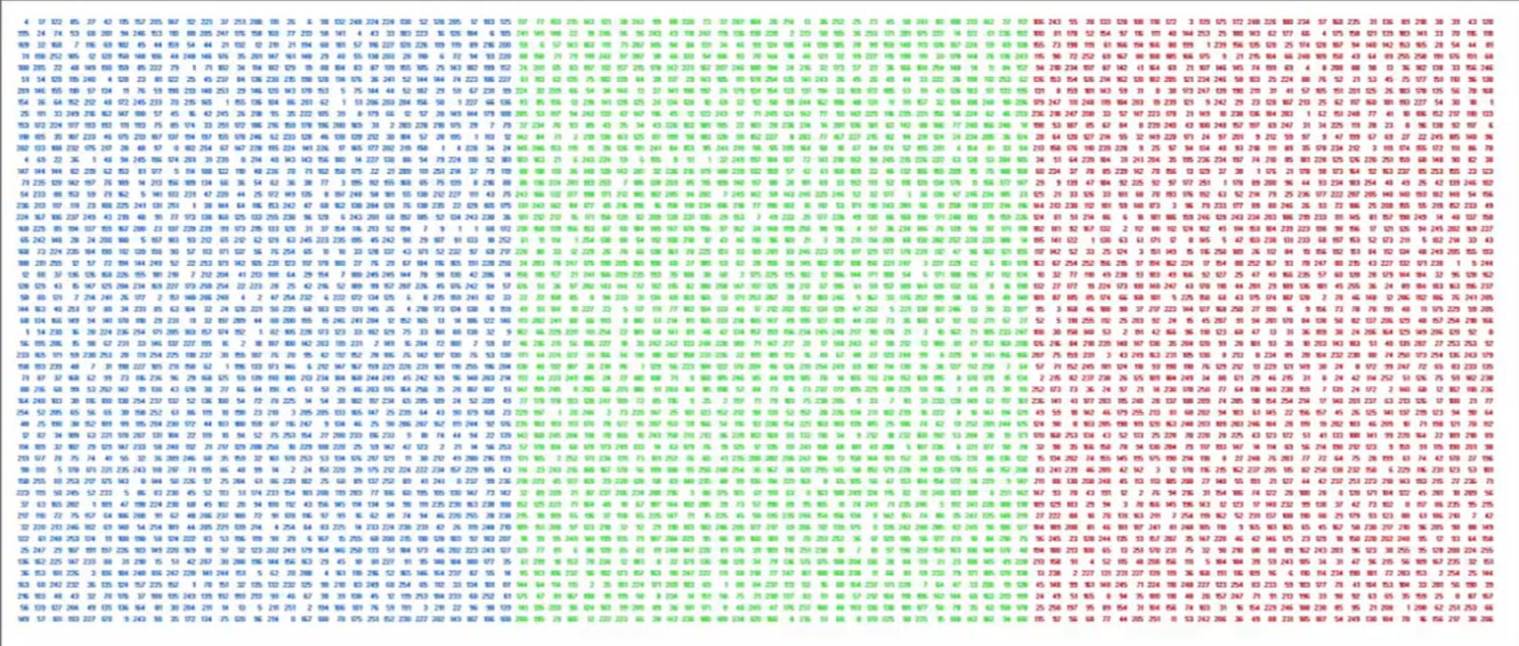
3-dimensional arrays, that's all colored images are. Another type of image that we'll encounter in computer vision tasks is grayscale images. Grayscale images take the three color values for each pixel and condense the information into one value; making the image array flat with the dimensions MxN. There are many variants of grayscale each using different proportions of the R, G & B values. The default grayscale variant in OpenCV uses the following formula:
X = 0.299 R + 0.587 G + 0.114 B
OpenCV
OpenCV is an open-source computer vision library that is used to perform image analysis, processing, manipulation and much more. It is rather easy to learn, you don't need to be a machine learning expert, you don't even need to be that good at Python to get started.
OpenCV can be easily installed from PyPI using pip:
pip install opencv-python
If that doesn't work try pip3 install opencv-python or python -m pip install opencv-python.
So now that we have installed OpenCV, let's load an image and display it. But before we can do that we have to import the module. A weird thing to note about the OpenCV module is that it is referred to as cv2 rather than opencv-python or opencv.
import cv2
To read an image from local storage we use the cv2.imread(path, flag) method. It takes two arguments, the first argument path specifies the location of the image, the argument flag is optional and is used to specify the format in which we want to load the object. There are three flags:
cv2.IMREAD_COLORor1: It loads the image in the BGR 8-bit format ignoring the alpha channel or the transparency values.cv2.IMREAD_GRAYSCALEor0: Used to load the image as a grayscale image.cv2.IMREAD_UNCHANGEDor-1: Loads the image as it is, with the alpha channel.
You can find the list of all filetypes supported by imread() method here.
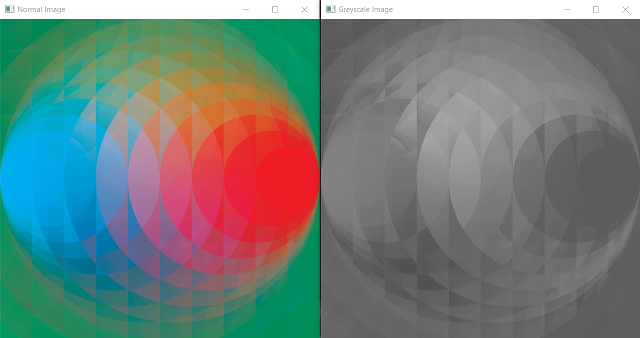
Let's try loading our image without any flag and then as a grayscale image.
normal_image = cv2.imread('images/ripple.jpg')
greyscale_image = cv2.imread('images/ripple.jpg', 0)
This code will execute without errors but we won't get any outputs. To see what we've just loaded we'll need to use the imshow(winname, img) method. The imshow() method creates a window with the name winname that displays the image img.
cv2.imshow("Normal Image", normal_image)
cv2.imshow("Greyscale Image", greyscale_image)
This code will create two windows that display the normal and grayscale version of the image but the windows will disappear before we'll be able to observe them. To keep them alive we'll use two more lines of code.
# waits the specified amount of time(in milliseconds) for a key press.
cv2.waitKey(0) # will wait for infinite amount of time if '0' is specified.
cv2.destroyAllWindows() # manually closing all windows
Executing these 7 lines of code will create two windows like this:
Color Models
RGB
Based on the primitive color theory of human perception, the RGB color model predates the electronic age. It is an additive color model in which colors are represented in terms of their red, green, and blue components. RGB describes a color as a tuple of three components. Each component can take a value between 0 and 255, where the tuple (0, 0, 0) represents black and (255, 255, 255) represents white.
OpenCV already has the three separate components albeit in the reverse order, BGR.
The reason the early developers at OpenCV chose BGR color format is that back then BGR color format was popular among camera manufacturers and software providers. E.g. in Windows, when specifying color value using COLORREF they use the BGR format 0x00bbggrr.
We can split these components by either slicing the array:
B = image[:,:,0]
G = image[:,:,1]
R = image[:,:,2]
or by using the cv2.split() method:
B, G, R = cv2.split(image)
Let's display these components using imshow()
cv2.imshow("Blue Channel", B)
cv2.imshow("Green Channel", G)
cv2.imshow("Red Channel", R)
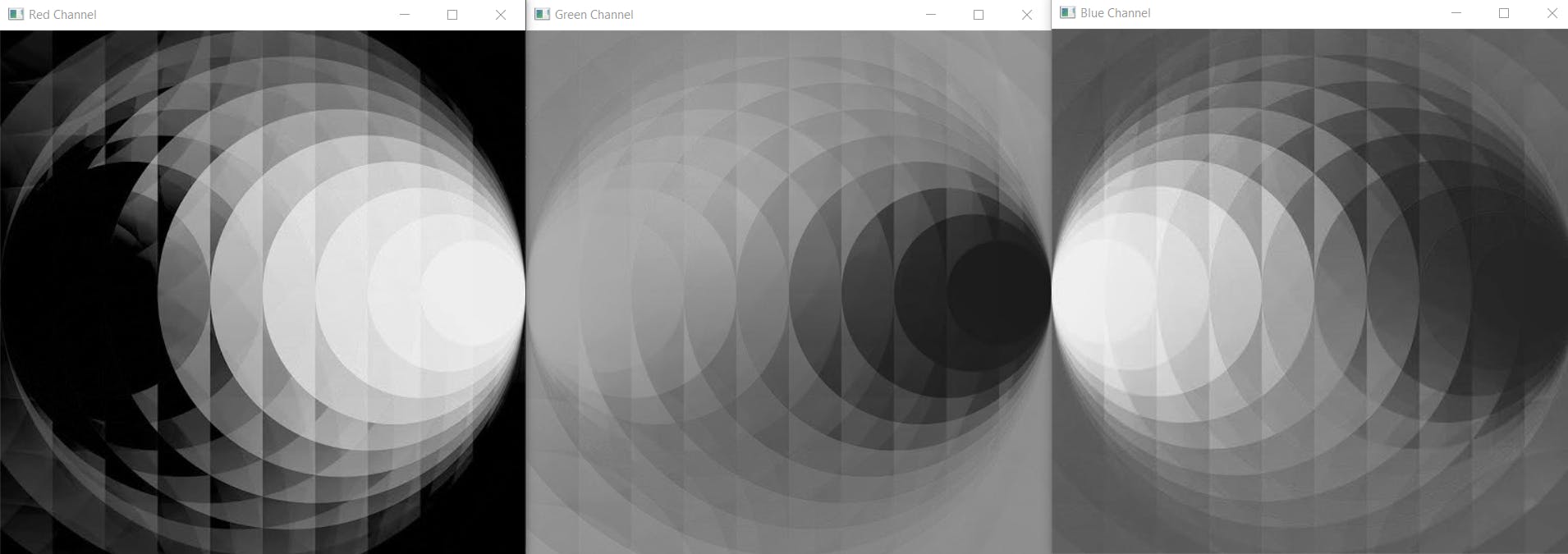
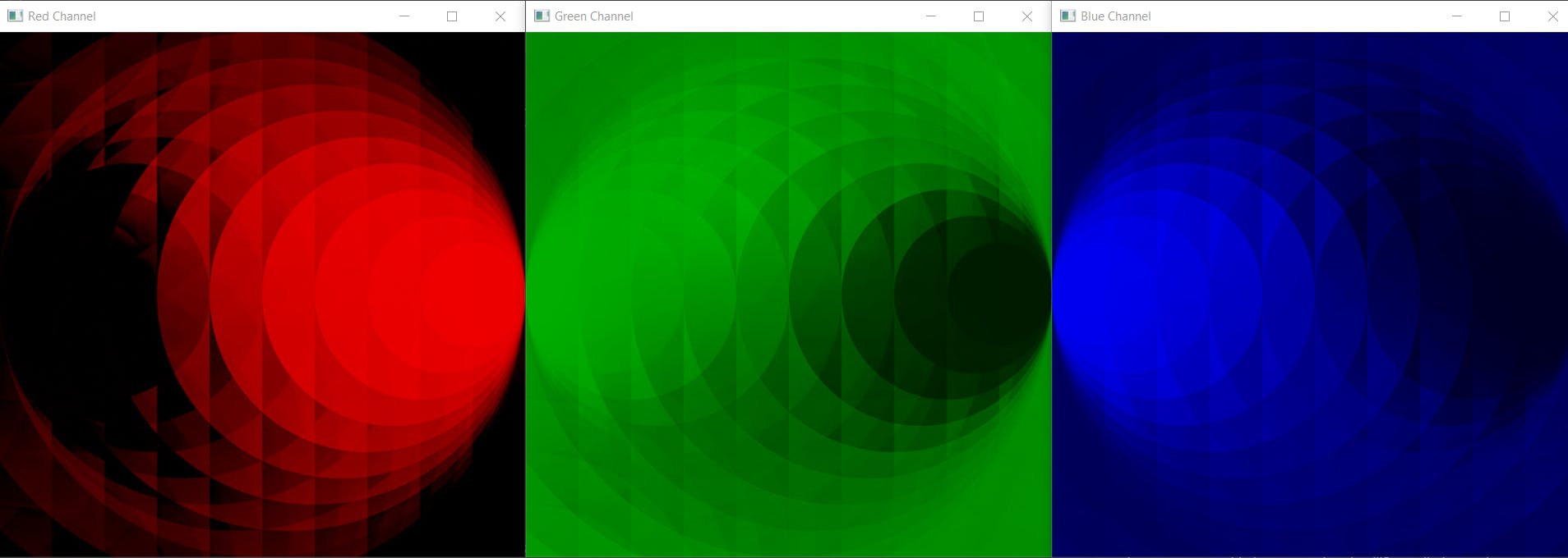
Huh, what went wrong? Well, nothing. Our image was successfully split into its three components, it's just that it went from being a 3xMxN array to three MxN arrays. And OpenCV treats all 2D arrays as grayscale. To visually see the three color components we'll need to add the missing two components with values zero.
import numpy as np
# creating an array of zeros with the dimensions of the input image
zeros = np.zeros(image.shape[:2], dtype = 'uint8')

cv2.imshow("Blue Channel", cv2.merge([B, zeros, zeros]))
cv2.imshow("Green Channel", cv2.merge([zeros, G, zeros]))
cv2.imshow("Red Channel", cv2.merge([zeros, zeros, R]))
The RGB color model is mainly used for the sensing, representation, and display of images in electronic systems, though it has also been used in conventional photography. But the human eye perceives color and brightness differently than the typical RGB sensors. When twice the number of photons of a particular wavelength hit the sensor of a digital camera, it creates twice the signal, i.e., a linear relationship. This is not how human eyes work, we perceive double the amount of light as only a fraction brighter, i.e., a non-linear relationship. Similarly our eyes are also much more sensitive to changes in darker tones than brighter tones.
HSV
The HSV model was created by computer graphic researchers in the 1970s in an attempt to better model how the human visual system perceives color attributes. Most of the color selector tools in multimedia applications make use of this model.
HSV model separates the color information (Hue) from the intensity (Saturation) and lighting (Value). Separating these values allows us to set better threshold values that work regardless of the lighting changes. Even by singling out only the hue values, we are able to obtain a very meaningful representation of the base color that works much better than RGB. The end result is a more robust color thresholding using simpler parameters.
Hue is a continuous representation of color so 0 and 360 are the same hue. Geometrically you can picture the HSV color space as a cylinder or a cone with H being the degree, saturation being the distance from the center, and value being the height.

To convert OpenCV's default BGR arrays into an HSV image we can use the cv2.cvtcolor(img, code) method that takes two arguments: the source image array img and the code that indicates the conversion type. You can find a list of all conversion codes here.
hsv_image = cv2.cvtColor(image, cv2.COLOR_RGB2HSV)

cv2.imshow("HSV Image", hsv_image)
cv2.imshow("Hue Channel", hsv_image[:, :, 0])
cv2.imshow("Saturation Channel", hsv_image[:, :, 1])
cv2.imshow("Value Channel", hsv_image[:, :, 2])
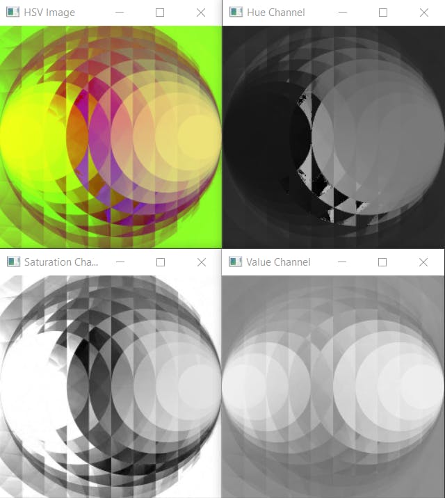
Now, this doesn't make intuitive sense as the RGB components did, but it isn't supposed to. The kind of image manipulation that we just performed happens behind the scenes in our brain. There's all sorts of math happening in there that allows us to do straightforward things like detecting contours, it's just that we're not doing it consciously.
Finding Nemo
Armed with our newfound rudimentary knowledge of computer vision we now set out to find Nemo. To accomplish this we will make use of the HSV color model and create a "mask". But before we start making our mask, let's understand what it is.
A mask is a very basic filter that sets some of the pixel values in an image to zero, or some other background value. Simply put, it allows you to hide some portions of an image and to reveal some portions. We'll be using it as an image segmentation method to separate the clownfish from the background. Beyond segmentation, masking has widespread applications and is used in many types of image processing, including motion detection, edge detection, and noise reduction.
First of all we'll need to load the image
image = cv2.imread("images/fish.jpg")
Displaying 3 windows of HD images on one screen isn't feasible, so we'll scale it scale down before converting to HSV. We can manually define the size of the image using the cv2.resize(image, size_tuple) method:
resized_images = cv2.resize(image, (512, 228))
or scale it down using scaling factors fx and fy:
resized_image = cv2.resize(image, None, fx=.4, fy=.4)

hsv_image = cv2.cvtColor(resized_image, cv2.COLOR_BGR2HSV)
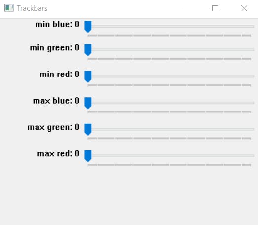
To find the range of hue values corresponding to the orange and white colors of the fish we'll need to do a lot of trial and error. Rather than repeatedly stopping the code to tweak the values we'll use value sliders to vary the range during runtime. To do this we'll create a resizable namedWindow and add a bunch Trackbar objects using the createTrackbar('trackbar_name', 'window_name', range_start, range_end, on_change) method. The Trackbar objects require an on_change function that is called when the slider is moved but we are not going to need this so we'll simply create a redundant function placeholder() that does nothing.
def placeholder(x):
    pass

cv2.namedWindow('Trackbars', cv2.WINDOW_NORMAL)
cv2.createTrackbar('min blue', 'Trackbars', 0, 255, placeholder)
cv2.createTrackbar('min green', 'Trackbars', 0, 255, placeholder)
cv2.createTrackbar('min red', 'Trackbars', 0, 255, placeholder)
cv2.createTrackbar('max blue', 'Trackbars', 0, 255, placeholder)
cv2.createTrackbar('max green', 'Trackbars', 0, 255, placeholder)
cv2.createTrackbar('max red', 'Trackbars', 0, 255, placeholder)
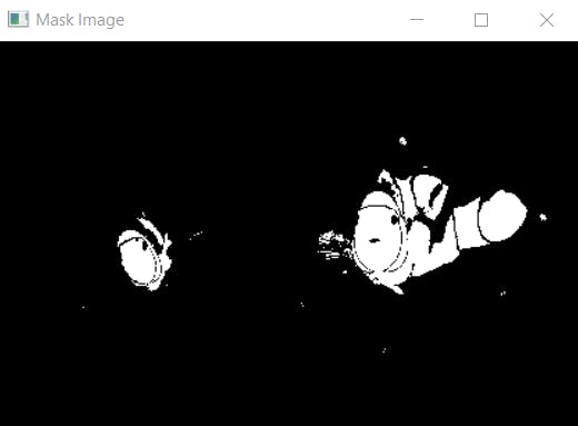
Now that we have a way to find the range of hues, let's put it to work. To see the real-time effects of the hue sliders we'll need to continuously update the mask output screen. We'll do this using a while loop break out of it using the ESC key which has the ASCII value of 27. We fetch the positions of the sliders from our Trackbar window using the getTrackbarPos('trackbar_name', 'window_name') method and pass them to inRange(hsv_image, hue_thresh_min_tuple, hue_thresh_max_tuple). This creates a mask that filters out the pixel with hue values that don't lie within the defined thresholds. The mask creates a black-and-white image in which only the pixels within the hue range are illuminated, i.e., colored white.
We print the final values of the hue range so we can hardcode them for our final masks.
 cv2.imshow('Base Image', resized_image)
 cv2.imshow('HSV Image', hsv_image)

while True:
    # fetching the threshold values from the sliders
    min_blue = cv2.getTrackbarPos('min blue', 'Trackbars')
    min_green = cv2.getTrackbarPos('min green', 'Trackbars')
    min_red = cv2.getTrackbarPos('min red', 'Trackbars')
    max_blue = cv2.getTrackbarPos('max blue', 'Trackbars')
    max_green = cv2.getTrackbarPos('max green', 'Trackbars')
    max_red = cv2.getTrackbarPos('max red', 'Trackbars')

    mask = cv2.inRange(hsv_image, (min_blue, min_green, min_red), (max_blue, max_green, max_red))

    # showing the mask image
    cv2.imshow('Mask Image', mask)
    # checking if the ESC key is pressed to break out of loop
    key = cv2.waitKey(10)
    if key == 27:
        break


print(f'min blue {min_blue}  min green {min_green} min red {min_red}')
print(f'max blue {max_blue}  max green {max_green} max red {max_red}')
#destroying all windows
cv2.destroyAllWindows()
Similarly, using the sliders we find out the hue threshold for the white as well. We obtain the final mask by combining the two.
    mask_orange = cv2.inRange(hsv_image, orange_min, orange_max)
    mask_white = cv2.inRange(hsv_image, white_min, white_max)
    final_mask = mask_orange + mask_white
Using this combined mask gives us
And if we want to add the color back in, we can do so by masking the resized RGB image using our final mask. The bitwise_and() method basically does the logical "and" operation wherever the mask is white. Simply put, white + any color = the same color and black + any color = black. If that doesn't make sense, don't fret about it we'll look into bitwise operations in the image manipulation post.
output = cv2.bitwise_and(resized_image, resized_image, mask=final_mask)
cv2.imshow('Mask Image', output)
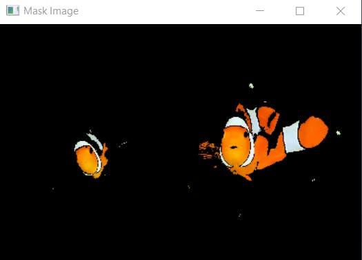
And there you have it, finding Nemo using basic color masking.